Optimize custom ops for GPUs with Mojo

Arthur Evans

Technical Writer

Brad Larson

Product Manager

custom-ops

max-graph

mojo

gpu

Building high-performance AI workloads for GPUs can be a daunting task, but Modular simplifies the experience with our custom op API that allows you to build graph operators for both GPUs and CPUs. In this tutorial, we'll teach you some strategies you can use to improve the performance of your GPU custom ops written in Mojo.

For demonstration purposes, we'll show you how to incrementally improve the performance of a custom matrix multiplication (matmul) op. We're not teaching you how to build a matmul op, because MAX already contains leading-edge implementations of matmul that you can use with the MAX graph API. Rather, we're using a basic matmul operation (AKA "GPU kernel") to teach you GPU programming strategies that might help with your other GPU code written in Mojo.

This page also isn't meant to teach you Mojo. For that, see the Mojo get started tutorial.

As you progress through this tutorial, you'll learn the following:

• How to define a custom matrix multiplication operation for a MAX graph.
• How to use of Mojo high-performance GPU programming abstractions to progressively optimize a matrix multiplication.
• How to access GPU hardware features, like Tensor Cores, from MAX.

Let's get started.

Requirements

Mac

Linux

WSL

GPU

To use a GPU, ensure your system meets these GPU requirements.

Run and compare the results

To get a sense of how each implementation of the custom op (kernel) performs, download the code and run the benchmark script:

1. Get the example code from GitHub:

   git clone https://github.com/modular/modular.git

   git clone https://github.com/modular/modular.git

2. If you don't have it, install pixi:

   curl -fsSL https://pixi.sh/install.sh | sh

   curl -fsSL https://pixi.sh/install.sh | sh

   Then restart your terminal for the changes to take effect.

3. Run all the matmul examples:

   cd modular/examples/custom_ops
   
   pixi run python matrix_multiplication.py

   cd modular/examples/custom_ops
   
   pixi run python matrix_multiplication.py

   As long as you have a compatible GPU, this will compile, run, and print the results of each matmul implementation that we'll discuss below.

4. Run the matmul benchmarks to see the impact of each optimization:

   pixi run mojo benchmarks.mojo --matmul

   pixi run mojo benchmarks.mojo --matmul

   This also runs each implementation but also benchmarks them and prints a comparison table. For example (this is running on a g5-2xlarge instance; your results will vary):

   ---------------------------------------------------------------------------------------------------------
   | name                       | met (ms)            | iters | GFLOPS/s           | GElems/s              |
   ---------------------------------------------------------------------------------------------------------
   | cpu/naive                  | 1647.331583         | 2     | 1.3183084343256959 | 0.0006415126201098278 |
   | gpu/naive                  | 2.842315817535545   | 422   | 764.0569378680037  | 0.37180386270949084   |
   | gpu/coalescing             | 1.0952283930000002  | 1000  | 1982.8659792606384 | 0.9648982867448362    |
   | gpu/tiled                  | 0.981560302         | 1000  | 2212.48874427279   | 1.076636858526905     |
   | gpu/tiled_register         | 0.39235773577501637 | 3058  | 5534.977195518529  | 2.693419559863031     |
   | gpu/block_tiled            | 0.38266733939393943 | 3135  | 5675.141033565811  | 2.7616258070879858    |
   | gpu/block_tiled_vectorized | 0.3684924709677419  | 3255  | 5893.447739370804  | 2.8678577807157195    |
   | gpu/tensor_core            | 0.18174263374734928 | 6602  | 11949.266252072646 | 5.814728103198369     |
   ---------------------------------------------------------------------------------------------------------

   ---------------------------------------------------------------------------------------------------------
   | name                       | met (ms)            | iters | GFLOPS/s           | GElems/s              |
   ---------------------------------------------------------------------------------------------------------
   | cpu/naive                  | 1647.331583         | 2     | 1.3183084343256959 | 0.0006415126201098278 |
   | gpu/naive                  | 2.842315817535545   | 422   | 764.0569378680037  | 0.37180386270949084   |
   | gpu/coalescing             | 1.0952283930000002  | 1000  | 1982.8659792606384 | 0.9648982867448362    |
   | gpu/tiled                  | 0.981560302         | 1000  | 2212.48874427279   | 1.076636858526905     |
   | gpu/tiled_register         | 0.39235773577501637 | 3058  | 5534.977195518529  | 2.693419559863031     |
   | gpu/block_tiled            | 0.38266733939393943 | 3135  | 5675.141033565811  | 2.7616258070879858    |
   | gpu/block_tiled_vectorized | 0.3684924709677419  | 3255  | 5893.447739370804  | 2.8678577807157195    |
   | gpu/tensor_core            | 0.18174263374734928 | 6602  | 11949.266252072646 | 5.814728103198369     |
   ---------------------------------------------------------------------------------------------------------

Introduction

AI models in MAX are built as computational graphs using the MAX graph API. MAX contains within it a powerful graph compiler that can take these graphs and optimize them for best performance on a wide range of hardware.

Each node in a MAX graph is defined by an operation that performs a calculation on zero or more inputs and produces one or more outputs. These inputs and outputs tend to be in the form of tensors, and the operations are usually data-parallel calculations that are accelerated on CPUs or GPUs. In MAX, these operations are written using Mojo, a Python-family language built for high-performance computation.

Matrix multiplications are key components in modern AI models, accounting for a sizable fraction of the GPU workload when running these models. Optimizations applied to matrix multiplication calculations can have a significant impact on the throughput of models on GPUs.

To review, a matrix multiplication involves multiplying two matrices, A and B, to produce a new matrix C.

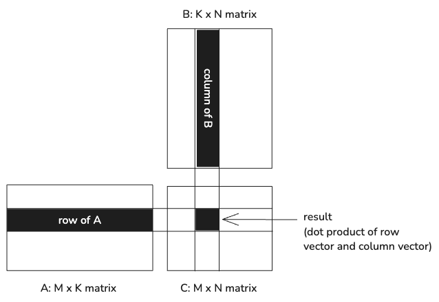
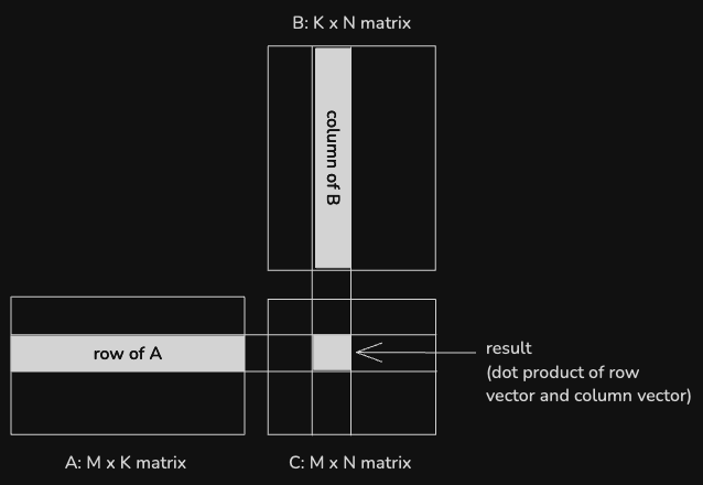
Each value in the output matrix is the dot product of a row from A and a column from B. In a worst case scenario, when multiplying an MxK matrix by a KxN matrix, calculating one output value requires loading 2 * K values and performing K floating-point multiplications.

Structure of the custom operation

The matrix multiplication algorithms demonstrated here are encapsulated within a custom MAX graph operation. AI models in MAX are built from a graph of operations like this, and in this case we're demonstrating one of these operations running in isolation. The matrix_multiplication.py file exercises seven different matrix multiplication algorithms using a single-operation graph and shows that the results of multiplying two random matrices are the same for each.

These results can be seen by running at the command line using

pixi run python matrix_multiplication.py

pixi run python matrix_multiplication.py

The single-operation graph is constructed using the following function:

🐍 Python

def matrix_multiplication(
    a: NDArray[np.float32],
    b: NDArray[np.float32],
    algorithm: str,
    session: InferenceSession,
    device: Device,
) -> Tensor:
    dtype = DType.float32

    a_tensor = Tensor.from_numpy(a).to(device)
    b_tensor = Tensor.from_numpy(b).to(device)

    with Graph(
        "matrix_multiplication_graph",
        input_types=[
            TensorType(dtype, shape=a_tensor.shape),
            TensorType(dtype, shape=b_tensor.shape),
        ],
    ) as graph:
        a_value, b_value = graph.inputs
        output = ops.custom(
            name="matrix_multiplication",
            values=[a_value, b_value],
            out_types=[
                TensorType(
                    dtype=a_value.tensor.dtype,
                    shape=[a_value.tensor.shape[0], b_value.tensor.shape[1]],
                )
            ],
            parameters={"algorithm": algorithm},
        )[0].tensor
        graph.output(output)

    print("Compiling...")
    model = session.load(graph)

    print("Executing...")
    result = model.execute(a_tensor, b_tensor)[0]
    return result.to(CPU())

def matrix_multiplication(
    a: NDArray[np.float32],
    b: NDArray[np.float32],
    algorithm: str,
    session: InferenceSession,
    device: Device,
) -> Tensor:
    dtype = DType.float32

    a_tensor = Tensor.from_numpy(a).to(device)
    b_tensor = Tensor.from_numpy(b).to(device)

    with Graph(
        "matrix_multiplication_graph",
        input_types=[
            TensorType(dtype, shape=a_tensor.shape),
            TensorType(dtype, shape=b_tensor.shape),
        ],
    ) as graph:
        a_value, b_value = graph.inputs
        output = ops.custom(
            name="matrix_multiplication",
            values=[a_value, b_value],
            out_types=[
                TensorType(
                    dtype=a_value.tensor.dtype,
                    shape=[a_value.tensor.shape[0], b_value.tensor.shape[1]],
                )
            ],
            parameters={"algorithm": algorithm},
        )[0].tensor
        graph.output(output)

    print("Compiling...")
    model = session.load(graph)

    print("Executing...")
    result = model.execute(a_tensor, b_tensor)[0]
    return result.to(CPU())

A single matrix_multiplication operation is used, and the algorithm variant is specified by the algorithm compile-time parameter.

The custom operation itself is defined in Mojo within the operations/matrix_multiplication.mojo file. The MatrixMultiplication struct hosts all of the setup code for taking in the matrix tensors, branching execution based on whether the operation is running on CPU or GPU, and then selecting and running a specific algorithm. Mojo supports compile-time specialization of code based on parameters like target hardware, and that is also extended here to user-supplied algorithm choice. Compiling only the code paths used for a particular piece of hardware avoids run-time branching and allows full utilization of an accelerator or CPU.

Each algorithm is contained within its own function in operations/matrix_multiplication.mojo. Next, we'll discuss how each works.

Matrix multiplication algorithms

The algorithms demonstrated in this example follow steps 1-6 in the progression detailed by Simon Boehm in his excellent blog post on writing performant matrix multiplications. Each algorithm is represented by a shortened parameter name from the following list:

1. naive: Naive matrix multiplication with no optimizations.
2. coalescing: Applying memory coalescing.
3. tiled: Reworking to use shared memory tiling.
4. tiled_register: Using shared memory tiling and register tiling.
5. block_tiled: Introducing block tiling.
6. block_tiled_vectorized: Block tiling with vectorized memory access.
7. tensor_core: Using Tensor Cores for matrix multiplication.

The last algorithm is not from Simon's original list, but shows how to access Tensor Core hardware using MAX in Mojo.

Each algorithm is meant to show a progressive improvement in performance of matrix multiplication on GPUs. To start with, the impact of each optimization can be seen by running a set of benchmarks against the algorithms in sequence:

pixi run mojo benchmarks.mojo --matmul

pixi run mojo benchmarks.mojo --matmul

The results on an NVIDIA A100 GPU for 32-bit floats and input matrices sized to 4096x4096 look like the following at the time this is written:

Algorithm	GFLOPS/s
naive	292
coalescing	2936
tiled	3943
tiled_register	7078
block_tiled	10661
block_tiled_vectorized	10663

The specific numbers may vary for your GPU, but the general progression should be the same.

Layouts and LayoutTensor

The matrix_multiplication custom operation uses layouts and LayoutTensor to represent the input and output matrices, so it's helpful to understand a little bit about these types before getting started.

A layout represents a mapping from a set of logical coordinates to a single, one-dimensional coordinate—such as an array index or memory offset. For example, a layout could represent a 2x6, row-major layout:

🔥 Mojo

my_layout = Layout.row_major(2, 6)
print_layout(my_layout)

my_layout = Layout.row_major(2, 6)
print_layout(my_layout)

       0    1    2    3    4    5
    +----+----+----+----+----+----+
 0  |  0 |  1 |  2 |  3 |  4 |  5 |
    +----+----+----+----+----+----+
 1  |  6 |  7 |  8 |  9 | 10 | 11 |
    +----+----+----+----+----+----+

       0    1    2    3    4    5
    +----+----+----+----+----+----+
 0  |  0 |  1 |  2 |  3 |  4 |  5 |
    +----+----+----+----+----+----+
 1  |  6 |  7 |  8 |  9 | 10 | 11 |
    +----+----+----+----+----+----+

A LayoutTensor consists of a layout and a pointer to memory. For example, if you create a LayoutTensor using the layout shown above, the value at (1, 1) is stored at memory offset 7.

A layout tensor can point to an existing buffer, or you can allocate memory to store the tensor data. One LayoutTensor you'll see a lot in the following sections is tile(), which returns a new LayoutTensor which is a subset of the original, but points to the same underlying data.

For example, you can extract a 2x2 tile of the above tensor:

🔥 Mojo

tile = my_tensor.tile[2, 2](0, 1)

tile = my_tensor.tile[2, 2](0, 1)

The layout of the extracted tile looks like this:

       0    1
    +----+----+
 0  |  2 |  3 |
    +----+----+
 1  |  8 |  9 |
    +----+----+

       0    1
    +----+----+
 0  |  2 |  3 |
    +----+----+
 1  |  8 |  9 |
    +----+----+

This just scratches the surface of layouts and LayoutTensor, which provide powerful tools for manipulating data and writing parallel algorithms.

Kernel 1: Naive matrix multiplication with no optimizations

The very first algorithm to start with is a "naive" matrix multiplication, one that expresses the problem but makes no attempt at optimizing for how GPUs actually work.

In Mojo, a basic matrix multiplication looks like the following:

🔥 Mojo

fn naive_matrix_multiplication[
    dtype: DType,
    a_layout: Layout,
    b_layout: Layout,
    c_layout: Layout,
    BM: Int,
    BN: Int,
](
    a: LayoutTensor[dtype, a_layout, MutableAnyOrigin],
    b: LayoutTensor[dtype, b_layout, MutableAnyOrigin],
    c: LayoutTensor[dtype, c_layout, MutableAnyOrigin],
):

    var M = a.dim(0)
    var N = b.dim(1)
    var K = b.dim(0)

    var row = block_dim.x * block_idx.x + thread_idx.x
    var col = block_dim.y * block_idx.y + thread_idx.y

    var dst_reg: c.element_type = 0

    if row < M and col < N:
        for k_index in range(K):
            dst_reg = dst_reg + a[row, k_index] * b[k_index, col]

    c[row, col] = dst_reg

fn naive_matrix_multiplication[
    dtype: DType,
    a_layout: Layout,
    b_layout: Layout,
    c_layout: Layout,
    BM: Int,
    BN: Int,
](
    a: LayoutTensor[dtype, a_layout, MutableAnyOrigin],
    b: LayoutTensor[dtype, b_layout, MutableAnyOrigin],
    c: LayoutTensor[dtype, c_layout, MutableAnyOrigin],
):

    var M = a.dim(0)
    var N = b.dim(1)
    var K = b.dim(0)

    var row = block_dim.x * block_idx.x + thread_idx.x
    var col = block_dim.y * block_idx.y + thread_idx.y

    var dst_reg: c.element_type = 0

    if row < M and col < N:
        for k_index in range(K):
            dst_reg = dst_reg + a[row, k_index] * b[k_index, col]

    c[row, col] = dst_reg

However, if you glance up at the benchmark table in the previous section, you'll see that the naive matrix multiplication is roughly only 2.7% as fast as sixth algorithm on our list. There's clearly a lot of upside if this core algorithm can be improved.

Kernel 2: Applying memory coalescing

As one quick optimization that has an outsized impact, global memory accesses can be coalesced by swapping the thread indices for columns and rows:

🔥 Mojo

var row = block_dim.y * block_idx.y + thread_idx.y
var col = block_dim.x * block_idx.x + thread_idx.x

var row = block_dim.y * block_idx.y + thread_idx.y
var col = block_dim.x * block_idx.x + thread_idx.x

With this change, adjacent threads access values in the same row of the input matrices, which are contiguous in memory.

This leads to an almost tenfold jump in benchmarks on A100.

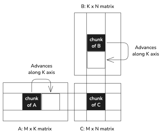
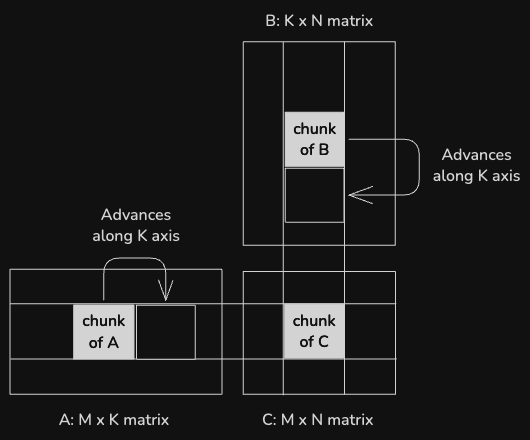
Kernel 3: Reworking to use shared memory tiling

Shared memory on the GPU is far faster to access than global memory, so a next step is to rework the matrix multiplication to tile the computation and load values into shared memory. The signature for this kernel is the same as the previous two, with the addition of a new BK parameter, representing the tile size along the K axis.

The input matrices A and B are loaded into shared memory in tiles of size BM x BK and BK x BN, respectively. Within the tile, values are accessed from shared memory, significantly reducing the memory access latency in between arithmetic operations. Since each value in shared memory is used by BK threads (32 in this case), this greatly reduces the number of reads from global memory.

This version corresponds to "Kernel 3: Shared Memory Cache-Blocking" in Simon's blog post.

Each thread is still computing a single output value, but it calculates a partial result for each tile worth of input data, and accumulates the partial results to calculate the final value.

We'll walk through the interesting part of the kernel.

The LayoutTensor tile() method provides a view to one tile of a tensor, without copying any data. It serves multiple purposes here. First, for the destination tile:

🔥 Mojo

var col = thread_idx.x % BN
var row = thread_idx.x // BN

var dst = c.tile[BM, BN](block_idx.y, block_idx.x)

var col = thread_idx.x % BN
var row = thread_idx.x // BN

var dst = c.tile[BM, BN](block_idx.y, block_idx.x)

The dst value is a view of the chunk of the output tensor that the current block is responsible for generating. dst is a 32x32 chunk of the output tensor, but instead of the 32x32 thread blocks used for previous kernels, this kernel is invoked with a one-dimensional thread block of 32*32 threads. The threads are mapped onto the output tile in row-major order, like this:

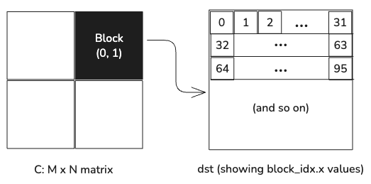
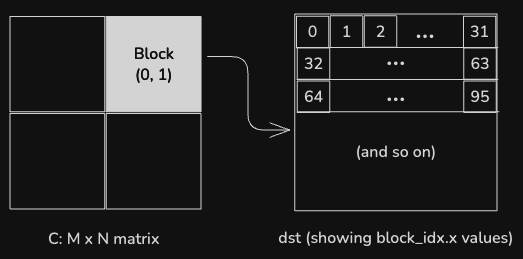
As in the previous example, accessing memory in this order is more efficient for the GPU, since it can coalesce adjacent memory accesses for adjacent threads in the same warp.

Next the kernel uses the LayoutTensorBuild struct (imported as tb for brevity) to allocate layout tensors in shared memory to hold cached chunks of the input tensors.

🔥 Mojo

var a_smem = tb[dtype]().row_major[BM, BK]().shared().alloc()
var b_smem = tb[dtype]().row_major[BK, BN]().shared().alloc()

var dst_reg: c.element_type = 0

var a_smem = tb[dtype]().row_major[BM, BK]().shared().alloc()
var b_smem = tb[dtype]().row_major[BK, BN]().shared().alloc()

var dst_reg: c.element_type = 0

The kernel then iterates across the input matrices, loading tiles into shared memory.

The copy_dram_to_sram_async() function deserves special note. This takes the place of the CUDA pattern of instructing each thread which value or values to copy to shared memory. The thread_layout parameter associates individual threads with values, and the function ensures efficient memory copies.

🔥 Mojo

for block in range(b.dim(0) // BK):
    alias load_a_layout = Layout.row_major(NUM_THREADS // BK, BK)
    alias load_b_layout = Layout.row_major(BK, NUM_THREADS // BK)

    var a_tile = a.tile[BM, BK](block_idx.y, block)
    var b_tile = b.tile[BK, BN](block, block_idx.x)

    copy_dram_to_sram_async[thread_layout=load_a_layout](a_smem, a_tile)
    copy_dram_to_sram_async[thread_layout=load_b_layout](b_smem, b_tile)

    async_copy_wait_all()

    barrier()

    @parameter
    for k in range(BK):
        dst_reg += a_smem[row, k] * b_smem[k, col]

    barrier()

for block in range(b.dim(0) // BK):
    alias load_a_layout = Layout.row_major(NUM_THREADS // BK, BK)
    alias load_b_layout = Layout.row_major(BK, NUM_THREADS // BK)

    var a_tile = a.tile[BM, BK](block_idx.y, block)
    var b_tile = b.tile[BK, BN](block, block_idx.x)

    copy_dram_to_sram_async[thread_layout=load_a_layout](a_smem, a_tile)
    copy_dram_to_sram_async[thread_layout=load_b_layout](b_smem, b_tile)

    async_copy_wait_all()

    barrier()

    @parameter
    for k in range(BK):
        dst_reg += a_smem[row, k] * b_smem[k, col]

    barrier()

The async_copy_wait_all() and barrier() calls ensure that all threads have completed their memory copies before proceeding to the next step, the inner loop, which accumulates the partial results for the current output tile. The @parameter for construct tells the compiler that this loop can be unrolled at compile time, since BK is a parameter, static at runtime.

Finally, after all of the tiles have been processed, the results are written to the output tensor.

🔥 Mojo

dst[row, col] += dst_reg

dst[row, col] += dst_reg

All together, this kernel improves overall performance by ~30% over the previous optimization.

Note: While faster on A100, this kernel may not show gains over the previous one on all GPUs.

Kernel 4: Using shared memory tiling and register tiling

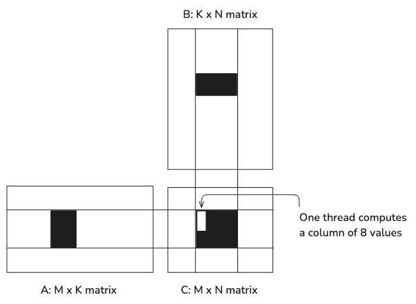
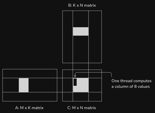
Expanding upon the advantages of using shared memory tiling, the partial results can be accumulated in tiled registers and then the final results transferred from there to global memory.

In this version, each thread is responsible for calculating multiple values of C, further reducing the memory bandwidth required for each calculation. Specifically, each thread calculates a column of 8 results:

This kernel adds another new parameter to the signature, TM, which specifies the size of the register tile. You'll notice the code looks very similar to the previous kernel, except that the results are stored to a register tile. Also, note that the inner loop is structured so that the thread uses a single value from B for all of the calculations for a single register tile.

Here's the interesting part of this kernel:

🔥 Mojo

var col = thread_idx.x % BN
var row = thread_idx.x // BN

var dst = c.tile[BM, BN](block_idx.y, block_idx.x).tile[TM, 1](row, col)

var a_smem = tb[dtype]().row_major[BM, BK]().shared().alloc()
var b_smem = tb[dtype]().row_major[BK, BN]().shared().alloc()

var dst_reg = tb[dtype]().layout[TM]().local().alloc()
dst_reg.copy_from(dst)

for block in range(b.dim(0) // BK):
    alias load_a_layout = Layout.row_major(NUM_THREADS // BK, BK)
    alias load_b_layout = Layout.row_major(BK, NUM_THREADS // BK)

    var a_tile = a.tile[BM, BK](block_idx.y, block)
    var b_tile = b.tile[BK, BN](block, block_idx.x)

    copy_dram_to_sram_async[thread_layout=load_a_layout](a_smem, a_tile)
    copy_dram_to_sram_async[thread_layout=load_b_layout](b_smem, b_tile)

    async_copy_wait_all()
    barrier()

    @parameter
    for k in range(BK):
        var a_tile = a_smem.tile[TM, 1](row, k)
        var b_tile = b_smem.tile[1, BN](k, 0)
        var b_val = b_tile[0, col]

        @parameter
        for t in range(TM):
            dst_reg[t] += a_tile[t, 0] * b_val

    barrier()

dst.copy_from(dst_reg)

var col = thread_idx.x % BN
var row = thread_idx.x // BN

var dst = c.tile[BM, BN](block_idx.y, block_idx.x).tile[TM, 1](row, col)

var a_smem = tb[dtype]().row_major[BM, BK]().shared().alloc()
var b_smem = tb[dtype]().row_major[BK, BN]().shared().alloc()

var dst_reg = tb[dtype]().layout[TM]().local().alloc()
dst_reg.copy_from(dst)

for block in range(b.dim(0) // BK):
    alias load_a_layout = Layout.row_major(NUM_THREADS // BK, BK)
    alias load_b_layout = Layout.row_major(BK, NUM_THREADS // BK)

    var a_tile = a.tile[BM, BK](block_idx.y, block)
    var b_tile = b.tile[BK, BN](block, block_idx.x)

    copy_dram_to_sram_async[thread_layout=load_a_layout](a_smem, a_tile)
    copy_dram_to_sram_async[thread_layout=load_b_layout](b_smem, b_tile)

    async_copy_wait_all()
    barrier()

    @parameter
    for k in range(BK):
        var a_tile = a_smem.tile[TM, 1](row, k)
        var b_tile = b_smem.tile[1, BN](k, 0)
        var b_val = b_tile[0, col]

        @parameter
        for t in range(TM):
            dst_reg[t] += a_tile[t, 0] * b_val

    barrier()

dst.copy_from(dst_reg)

This gives a nearly 80% improvement over the previous tiling implementation.

Kernel 5: Introducing block tiling

We can further increase the arithmetic intensity of the calculation using a 2-D block tiling strategy. In this kernel, each thread is responsible for calculating the output values for a TMxTN tile of the output tensor. (Where TM and TN and kernel parameters; in this case we're using 8x8 tiles.)

In addition to caching a block's worth of the A & B matrices in shared memory, each thread copies 8-unit vectors of the input matrices into local storage to further reduce memory access latency. Then it uses the outer_product_acc() function to calculate and accumulate the outer products of the two vectors.

🔥 Mojo

var partition_col = thread_idx.x % (BN // TN)
var partition_row = thread_idx.x // (BN // TN)

var dst = c.tile[BM, BN](block_idx.y, block_idx.x).tile[TM, TN](
    partition_row, partition_col
)

var a_smem = tb[dtype]().row_major[BM, BK]().shared().alloc()
var b_smem = tb[dtype]().row_major[BK, BN]().shared().alloc()

var dst_reg = tb[dtype]().row_major[TM, TN]().local().alloc()
dst_reg.copy_from(dst)
var a_reg = tb[dtype]().layout[TM]().local().alloc()
var b_reg = tb[dtype]().layout[TN]().local().alloc()

var ntiles = b.dim(0) // BK

for block in range(ntiles):
    alias load_a_layout = Layout.row_major(NUM_THREADS // BK, BK)
    alias load_b_layout = Layout.row_major(BK, NUM_THREADS // BK)
    var a_tile = a.tile[BM, BK](block_idx.y, block)
    var b_tile = b.tile[BK, BN](block, block_idx.x)
    copy_dram_to_sram_async[thread_layout=load_a_layout](a_smem, a_tile)
    copy_dram_to_sram_async[thread_layout=load_b_layout](b_smem, b_tile)

    async_copy_wait_all()
    barrier()

    @parameter
    for k in range(BK):
        var a_tile = a_smem.tile[TM, 1](partition_row, k)
        var b_tile = b_smem.tile[1, TN](k, partition_col)
        a_reg.copy_from(a_tile)
        b_reg.copy_from(b_tile)
        outer_product_acc(dst_reg, a_reg, b_reg)
    barrier()

dst.copy_from(dst_reg)

var partition_col = thread_idx.x % (BN // TN)
var partition_row = thread_idx.x // (BN // TN)

var dst = c.tile[BM, BN](block_idx.y, block_idx.x).tile[TM, TN](
    partition_row, partition_col
)

var a_smem = tb[dtype]().row_major[BM, BK]().shared().alloc()
var b_smem = tb[dtype]().row_major[BK, BN]().shared().alloc()

var dst_reg = tb[dtype]().row_major[TM, TN]().local().alloc()
dst_reg.copy_from(dst)
var a_reg = tb[dtype]().layout[TM]().local().alloc()
var b_reg = tb[dtype]().layout[TN]().local().alloc()

var ntiles = b.dim(0) // BK

for block in range(ntiles):
    alias load_a_layout = Layout.row_major(NUM_THREADS // BK, BK)
    alias load_b_layout = Layout.row_major(BK, NUM_THREADS // BK)
    var a_tile = a.tile[BM, BK](block_idx.y, block)
    var b_tile = b.tile[BK, BN](block, block_idx.x)
    copy_dram_to_sram_async[thread_layout=load_a_layout](a_smem, a_tile)
    copy_dram_to_sram_async[thread_layout=load_b_layout](b_smem, b_tile)

    async_copy_wait_all()
    barrier()

    @parameter
    for k in range(BK):
        var a_tile = a_smem.tile[TM, 1](partition_row, k)
        var b_tile = b_smem.tile[1, TN](k, partition_col)
        a_reg.copy_from(a_tile)
        b_reg.copy_from(b_tile)
        outer_product_acc(dst_reg, a_reg, b_reg)
    barrier()

dst.copy_from(dst_reg)

In the above benchmarks, this provides an additional 50% boost over the previous algorithm.

Kernel 6: Block tiling with vectorized memory access

As a final optimization to our block-tiling kernel, memory accesses can be vectorized to improve memory access bandwidth. The only new thing in this kernel is the use of the LayoutTensor.vectorize() method to produce vectorized views of the tensors, allowing multiple values to be copied as a single SIMD vector.

🔥 Mojo

alias simd_width = simdwidthof[dtype]()
var partition_col = thread_idx.x % (BN // TN)
var partition_row = thread_idx.x // (BN // TN)

var dst = c.tile[BM, BN](block_idx.y, block_idx.x).tile[TM, TN](
    partition_row, partition_col
)
var dst_vec = dst.vectorize[1, simd_width]()

var a_smem = tb[dtype]().col_major[BM, BK]().shared().alloc()
var b_smem = tb[dtype]().row_major[BK, BN]().shared().alloc()

var dst_reg = tb[dtype]().row_major[TM, TN]().local().alloc()
var dst_reg_vec = dst_reg.vectorize[1, simd_width]()
dst_reg_vec.copy_from(dst_vec)

var a_reg = tb[dtype]().layout[TM]().local().alloc()
var b_reg = tb[dtype]().layout[TN]().local().alloc()

var ntiles = b.dim(0) // BK

for block in range(ntiles):
    alias load_a_layout = Layout.row_major(NUM_THREADS // BK, BK)
    alias load_b_layout = Layout.row_major(BK, NUM_THREADS // BK)
    var a_tile = a.tile[BM, BK](block_idx.y, block)
    var b_tile = b.tile[BK, BN](block, block_idx.x)

    copy_dram_to_sram_async[thread_layout=load_a_layout](
        a_smem.vectorize[simd_width, 1](), a_tile.vectorize[simd_width, 1]()
    )
    copy_dram_to_sram_async[thread_layout=load_b_layout](
        b_smem.vectorize[1, simd_width](), b_tile.vectorize[1, simd_width]()
    )

    async_copy_wait_all()
    barrier()

    @parameter
    for k in range(BK):
        var a_tile = a_smem.tile[TM, 1](partition_row, k)
        var b_tile = b_smem.tile[1, TN](k, partition_col)
        a_reg.copy_from(a_tile)
        b_reg.copy_from(b_tile)

        outer_product_acc(dst_reg, a_reg, b_reg)

    barrier()

dst_vec.copy_from(dst_reg_vec)

alias simd_width = simdwidthof[dtype]()
var partition_col = thread_idx.x % (BN // TN)
var partition_row = thread_idx.x // (BN // TN)

var dst = c.tile[BM, BN](block_idx.y, block_idx.x).tile[TM, TN](
    partition_row, partition_col
)
var dst_vec = dst.vectorize[1, simd_width]()

var a_smem = tb[dtype]().col_major[BM, BK]().shared().alloc()
var b_smem = tb[dtype]().row_major[BK, BN]().shared().alloc()

var dst_reg = tb[dtype]().row_major[TM, TN]().local().alloc()
var dst_reg_vec = dst_reg.vectorize[1, simd_width]()
dst_reg_vec.copy_from(dst_vec)

var a_reg = tb[dtype]().layout[TM]().local().alloc()
var b_reg = tb[dtype]().layout[TN]().local().alloc()

var ntiles = b.dim(0) // BK

for block in range(ntiles):
    alias load_a_layout = Layout.row_major(NUM_THREADS // BK, BK)
    alias load_b_layout = Layout.row_major(BK, NUM_THREADS // BK)
    var a_tile = a.tile[BM, BK](block_idx.y, block)
    var b_tile = b.tile[BK, BN](block, block_idx.x)

    copy_dram_to_sram_async[thread_layout=load_a_layout](
        a_smem.vectorize[simd_width, 1](), a_tile.vectorize[simd_width, 1]()
    )
    copy_dram_to_sram_async[thread_layout=load_b_layout](
        b_smem.vectorize[1, simd_width](), b_tile.vectorize[1, simd_width]()
    )

    async_copy_wait_all()
    barrier()

    @parameter
    for k in range(BK):
        var a_tile = a_smem.tile[TM, 1](partition_row, k)
        var b_tile = b_smem.tile[1, TN](k, partition_col)
        a_reg.copy_from(a_tile)
        b_reg.copy_from(b_tile)

        outer_product_acc(dst_reg, a_reg, b_reg)

    barrier()

dst_vec.copy_from(dst_reg_vec)

From beginning to end, we've realized more than a 36X improvement in matrix multiplication speed within our MAX custom operation!

Kernel 7: Using Tensor Cores for matrix multiplication

Modern GPUs have dedicated hardware units for performing accelerated matrix multiplication called Tensor Cores. These Tensor Cores can perform matrix multiplications an order of magnitude or more faster than general purpose GPU hardware. However, they can be a challenge to work with.

MAX contains interfaces that make it more ergonomic to program these dedicated hardware units. The following is an example of how to perform the same calculation as the above, only on a Tensor Core:

🔥 Mojo

fn tensor_core_matrix_multiplication[
    dtype: DType,
    layout_a: Layout,
    layout_b: Layout,
    layout_c: Layout,
    BM: Int,
    BN: Int,
    BK: Int,
    WM: Int,
    WN: Int,
    MMA_M: Int,
    MMA_N: Int,
    MMA_K: Int,
](
    A: LayoutTensor[dtype, layout_a, MutableAnyOrigin],
    B: LayoutTensor[dtype, layout_b, MutableAnyOrigin],
    C: LayoutTensor[dtype, layout_c, MutableAnyOrigin],
):
    alias M = C.shape[0]()
    alias N = C.shape[1]()
    alias K = A.shape[1]()

    var warp_id = thread_idx.x // WARP_SIZE

    warp_y = warp_id // (BN // WN)
    warp_x = warp_id % (BN // WN)

    C_warp_tile = C.tile[BM, BN](block_idx.y, block_idx.x).tile[WM, WN](
        warp_y, warp_x
    )

    mma_op = TensorCore[A.dtype, C.dtype, Index(MMA_M, MMA_N, MMA_K)]()

    A_sram_tile = tb[A.dtype]().row_major[BM, BK]().shared().alloc()
    B_sram_tile = tb[B.dtype]().row_major[BK, BN]().shared().alloc()

    c_reg = (
        tb[C.dtype]()
        .row_major[WM // MMA_M, (WN * 4) // MMA_N]()
        .local()
        .alloc()
        .fill(0)
    )

    for k_i in range(K // BK):
        barrier()

        A_dram_tile = A.tile[BM, BK](block_idx.y, k_i)
        B_dram_tile = B.tile[BK, BN](k_i, block_idx.x)

        copy_dram_to_sram_async[thread_layout = Layout.row_major(4, 8)](
            A_sram_tile.vectorize[1, 4](), A_dram_tile.vectorize[1, 4]()
        )
        copy_dram_to_sram_async[thread_layout = Layout.row_major(4, 8)](
            B_sram_tile.vectorize[1, 4](), B_dram_tile.vectorize[1, 4]()
        )

        async_copy_wait_all()
        barrier()

        A_warp_tile = A_sram_tile.tile[WM, BK](warp_y, 0)
        B_warp_tile = B_sram_tile.tile[BK, WN](0, warp_x)

        @parameter
        for mma_k in range(BK // MMA_K):

            @parameter
            for mma_m in range(WM // MMA_M):

                @parameter
                for mma_n in range(WN // MMA_N):
                    c_reg_m_n = c_reg.tile[1, 4](mma_m, mma_n)

                    A_mma_tile = A_warp_tile.tile[MMA_M, MMA_K](mma_m, mma_k)
                    B_mma_tile = B_warp_tile.tile[MMA_K, MMA_N](mma_k, mma_n)

                    a_reg = mma_op.load_a(A_mma_tile)
                    b_reg = mma_op.load_b(B_mma_tile)

                    var d_reg_m_n = mma_op.mma_op(
                        a_reg,
                        b_reg,
                        c_reg_m_n,
                    )

                    c_reg_m_n.copy_from(d_reg_m_n)

    @parameter
    for mma_m in range(WM // MMA_M):

        @parameter
        for mma_n in range(WN // MMA_N):
            var C_mma_tile = C_warp_tile.tile[MMA_M, MMA_N](mma_m, mma_n)
            var c_reg_m_n = c_reg.tile[1, 4](mma_m, mma_n)
            mma_op.store_d(C_mma_tile, c_reg_m_n)

fn tensor_core_matrix_multiplication[
    dtype: DType,
    layout_a: Layout,
    layout_b: Layout,
    layout_c: Layout,
    BM: Int,
    BN: Int,
    BK: Int,
    WM: Int,
    WN: Int,
    MMA_M: Int,
    MMA_N: Int,
    MMA_K: Int,
](
    A: LayoutTensor[dtype, layout_a, MutableAnyOrigin],
    B: LayoutTensor[dtype, layout_b, MutableAnyOrigin],
    C: LayoutTensor[dtype, layout_c, MutableAnyOrigin],
):
    alias M = C.shape[0]()
    alias N = C.shape[1]()
    alias K = A.shape[1]()

    var warp_id = thread_idx.x // WARP_SIZE

    warp_y = warp_id // (BN // WN)
    warp_x = warp_id % (BN // WN)

    C_warp_tile = C.tile[BM, BN](block_idx.y, block_idx.x).tile[WM, WN](
        warp_y, warp_x
    )

    mma_op = TensorCore[A.dtype, C.dtype, Index(MMA_M, MMA_N, MMA_K)]()

    A_sram_tile = tb[A.dtype]().row_major[BM, BK]().shared().alloc()
    B_sram_tile = tb[B.dtype]().row_major[BK, BN]().shared().alloc()

    c_reg = (
        tb[C.dtype]()
        .row_major[WM // MMA_M, (WN * 4) // MMA_N]()
        .local()
        .alloc()
        .fill(0)
    )

    for k_i in range(K // BK):
        barrier()

        A_dram_tile = A.tile[BM, BK](block_idx.y, k_i)
        B_dram_tile = B.tile[BK, BN](k_i, block_idx.x)

        copy_dram_to_sram_async[thread_layout = Layout.row_major(4, 8)](
            A_sram_tile.vectorize[1, 4](), A_dram_tile.vectorize[1, 4]()
        )
        copy_dram_to_sram_async[thread_layout = Layout.row_major(4, 8)](
            B_sram_tile.vectorize[1, 4](), B_dram_tile.vectorize[1, 4]()
        )

        async_copy_wait_all()
        barrier()

        A_warp_tile = A_sram_tile.tile[WM, BK](warp_y, 0)
        B_warp_tile = B_sram_tile.tile[BK, WN](0, warp_x)

        @parameter
        for mma_k in range(BK // MMA_K):

            @parameter
            for mma_m in range(WM // MMA_M):

                @parameter
                for mma_n in range(WN // MMA_N):
                    c_reg_m_n = c_reg.tile[1, 4](mma_m, mma_n)

                    A_mma_tile = A_warp_tile.tile[MMA_M, MMA_K](mma_m, mma_k)
                    B_mma_tile = B_warp_tile.tile[MMA_K, MMA_N](mma_k, mma_n)

                    a_reg = mma_op.load_a(A_mma_tile)
                    b_reg = mma_op.load_b(B_mma_tile)

                    var d_reg_m_n = mma_op.mma_op(
                        a_reg,
                        b_reg,
                        c_reg_m_n,
                    )

                    c_reg_m_n.copy_from(d_reg_m_n)

    @parameter
    for mma_m in range(WM // MMA_M):

        @parameter
        for mma_n in range(WN // MMA_N):
            var C_mma_tile = C_warp_tile.tile[MMA_M, MMA_N](mma_m, mma_n)
            var c_reg_m_n = c_reg.tile[1, 4](mma_m, mma_n)
            mma_op.store_d(C_mma_tile, c_reg_m_n)

Conclusion

In this tutorial, we've demonstrated how to create a custom MAX graph operation that performs matrix multiplication using various algorithms and run that on a GPU. We ran benchmarks of each algorithm, showing the performance benefits of various algorithmic improvements. Each improvement was described in detail, showing pathways to get the most speed out of modern GPUs using MAX and Mojo.

Next Steps

• Follow our tutorial for building a custom operation from scratch.

• See the GPU programming page in the Mojo manual.

• See the gpu module for detail on Mojo's GPU programming functions and types, and the documentation on @compiler.register shows how to register custom graph operations.

• Join our Modular Forum and Discord community to share your experiences and get support.

We're excited to see what you'll build with MAX! Share your projects and experiences with us using #ModularAI on social media.

Did this tutorial work for you?

Thank you! We'll create more content like this.

Thank you for helping us improve!

😔 What went wrong?

Some code doesn’t work

It's missing a step; I don't know what to do

I don't understand the purpose

Other

Submit